Stability as a foundation of machine learning

Cross-posted at offconvex.org.

Central to machine learning is our ability to relate how a learning algorithm fares on a sample to its performance on unseen instances. This is called generalization.

In this post, I will describe a purely algorithmic approach to generalization. The property that makes this possible is stability. An algorithm is stable, intuitively speaking, if its output doesn’t change much if we perturb the input sample in a single point. We will see that this property by itself is necessary and sufficient for generalization.

Example: Stability of the Perceptron algorithm

Before we jump into the formal details, let’s consider a simple example of a stable algorithm: The Perceptron, aka stochastic gradient descent for learning linear separators! The algorithm aims to separate two classes of points (here circles and triangles) with a linear separator. The algorithm starts with an arbitrary hyperplane. It then repeatedly selects a single example from its input set and updates its hyperplane using the gradient of a certain loss function on the chosen example. How bad might the algorithm screw up if we move around a single example? Let’s find out.

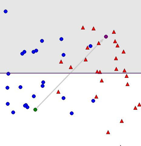
Step 1/30. Click to advance.
The animation shows two runs of the Perceptron algorithm for learning a linear separator on two data sets that differ in the one point marked green in one data set and purple in the other. The perturbation is indicated by an arrow. The shaded green region shows the difference in the resulting two hyperplanes after some number of steps.

As we can see by clicking impatiently through the example, the algorithm seems pretty stable. Even if we substantially move the first example it encounters, the hyperplane computed by the algorithm changes only slightly. Neat. (You can check out the code here.)

Empirical risk jargon

Let’s introduce some terminology to relate the behavior of an algorithm on a sample to its behavior on unseen instances. Imagine we have a sample $S=(z_1,\dots,z_n)$ drawn i.i.d. from some unknown distribution $D$. There’s a learning algorithm $A(S)$ that takes $S$ and produces some model (e.g., the hyperplane in the above picture). To quantify the quality of the model we crank out a loss function $\ell$ with the idea that $\ell(A(S), z)$ describes the loss of the model $A(S)$ on one instance $z$. The empirical risk or training error of the algorithm is defined as:

$R_S = \frac1n \sum_{i=1}^n \ell(A(S), z_i)$

This captures the average loss of the algorithm on the sample on which it was trained. To quantify out-of-sample performance, we define the risk of the algorithm as:

$R = \mathop{\mathbb{E}}_{z\sim D}\left[ \ell(A(S), z) \right]$

The difference between risk and empirical risk $R - R_S$ is called generalization error. You will sometimes encounter that term as a synonym for risk, but I find that confusing. We already have a perfectly short and good name for the risk $R$. Always keep in mind the following tautology

$R = R_S + (R-R_S).$

Operationally, it states that if we manage to minimize empirical risk all that matters is generalization error.

A fundamental theorem of machine learning

I probably shouldn’t propose fundamental theorems for anything really. But if I had to, this would be the one I’d suggest for machine learning:

In expectation, generalization equals stability.

Somewhat more formally, we will encounter a natural measure of stability, denoted $\Delta$ such that the difference between risk and empirical risk in expectation equals $\Delta.$ Formally,

$\mathbb{E}[R - R_S] = \Delta$

Deferring the exact definition of $\Delta$ to the proof, let’s think about this for a second. What I find so remarkable about this theorem is that it turns a statistical problem into a purely algorithmic one: All we need for generalization is an algorithmic notion of robustness. Our algorithm’s output shouldn’t change much if perturb one of the data points. It’s almost like a sanity check. Had you coded up an algorithm and this wasn’t the case, you’d probably go look for a bug.

Proof

Consider two data sets of size $n$ drawn independently of each other: [ S = (z_1,\dots,z_n), \qquad S’=(z_1’,\dots,z_n’) ] The idea of taking such a ghost sample $S’$ is quite old and already arises in the context of symmetrization in empirical process theory. We’re going to couple these two samples in one point by defining [ S^i = (z_1,\dots,z_{i-1},z_i’,z_{i+1},\dots,z_n),\qquad i = 1,\dots, n. ] It’s certainly no coincidence that $S$ and $S^i$ differ in exactly one element. We’re going to use this in just a moment.

By definition, the expected empirical risk equals

$\mathbb{E}[R_S] = \mathbb{E}\left[ \frac1n \sum_{i=1}^n \ell(A(S), z_i) \right].$

Contrasting this to how the algorithm fares on unseen examples, we can rewrite the expected risk using our ghost sample as:

$\mathbb{E}[R] = \mathbb{E}\left[ \frac1n \sum_{i=1}^n \ell(A(S), \color{red}{z_i'}) \right]$

All expectations we encounter are over both $S$ and $S’$. By linearity of expectation, the difference between expected risk and expected empirical risk equals

$\mathbb{E}[R - R_S] = \frac1n \sum_{i=1}^n \mathbb{E}\left[\ell(A(S), \color{red}{z_i'})-\ell(A(S), z_i)\right].$

It is tempting now to relate the two terms inside the expectation to the stability of the algorithm. We’re going to do exactly that using mathematics’ most trusted proof strategy: pattern matching. Indeed, since $z_i$ and $z_i’$ are exchangeable, we have

$\mathbb{E}[\ell(A(S), z_i)] = \mathbb{E}[\ell(A(S^i), z_i')] = \mathbb{E}[\ell(A(S), z_i')] - \delta_i,$

where $\delta_i$ is defined to make the second equality true:

$\delta_i = \mathbb{E}[\ell(A(\color{red}S), z_i')- \ell(A(\color{red}{S^i}), z_i')]$

Summing up $\Delta = (1/n)\sum_i \delta_i$, we have

$\mathbb{E}[ R - R_S ] = \Delta.$

The only thing left to do is to interpret the right hand side in terms of stability. Convince yourself that $\delta_i$ measures how differently the algorithm behaves on two data sets $S$ and $S’$ that differ in only one element.

Uniform stability

It can be difficult to analyze the expectation in the definition of $\Delta$ precisely. Fortunately, it is often enough to resolve the expectation by upper bounding it with suprema:

$|\Delta| \le \sup_{S,S'} \sup_{z} \left|\ell(A(S),z)-\ell(A(S'),z)\right|.$

The supremum runs over all valid data sets differing in only one element and all valid sample points $z$. This stronger notion of stability called uniform stability goes back to a seminal paper by Bousquett and Elisseeff.

I should say that you can find the above proof in the essssential stability paper by Shalev-Shwartz, Shamir, Srebro and Sridharan here.

Concentration from stability

The theorem we saw shows that expected empirical risk equals risk up to a correction that involves the stability of the algorithm. Can we also show that empirical risk is close to its expectation with high probability? Interestingly, we can by appealing to stability once again. I won’t spell out the details, but we can use the method of bounded differences to obtain strong concentration bounds. To apply the method we need a bounded difference condition which is just another word for stability. So, we’re really killing two birds with one stone by using stability not only to show that the first moment of the empirical risk is correct but also that it concentrates. The only wrinkle is that, as far as I know, the weak stability notion expressed by $\Delta$ is not enough to get concentration, but uniform stability (for sufficiently small difference) will do.

Applications of stability

There is much more that stability can do for us. We’ve only scratched on the surface. Here are some of the many applications of stability.

Regularization implies stability. Specifically, the minimizer of the empirical risk subject to an $\ell_2$-penalty is uniformly stable.
Stochastic gradient descent is stable provided that we don’t make too many steps.
Differential privacy is nothing but a strong stability guarantee. Any result ever proved about differential privacy is fundamentally about stability.
Differential privacy in turn has applications to preventing overfitting in adaptive data analysis.
Stability also has many beautiful applications and connections in statistics. I strongly encourage you to read Bin Yu’s beautiful overview paper on the topic.

Looking ahead, I’ve got at least two more posts planned on this.

In my next post I will go into the stability of stochastic gradient descent in detail. We will see a simple argument to show that stochastic gradient descent is uniformly stable. I will then work towards applying these ideas to the area of deep learning. We will see that stability can help us explain why even huge models sometimes generalize well and how we can make them generalize even better.

In a second post I will reflect on stability as a paradigm for reliable machine learning. The focus will be on how ideas from stability can help avoid overfitting and false discovery.