Pearson's polynomial

A 120 year old algorithm for learning mixtures of gaussians turns out to be optimal

So, how was math writing in 1894? I’d imagined it to be a lot like one of Nietzsche’s last diary entries except with nouns replaced by German fraktur symbols, impenetrable formalisms and mind-bending passive voice constructions. I was in for no small surprise when I started reading Karl Pearson’s Contributions to the Mathematical Theory of Evolution. The paper is quite enjoyable! The math is rigorous yet not overly formal. Examples and philosophical explanations motivate various design choices and definitions. A careful experimental evaluation gives credibility to the theory.

The utterly mind-boggling aspect of the paper however is not how well-written it is, but rather what Pearson actually did in it and how far ahead of his time he was. This is the subject of this post.

Pearson was interested in building a mathematical theory for evolutionary biology. In hindsight, his work is also one of the earliest contributions to the computational theory of evolution. This already strikes me as visionary as it remains a hot research area today. The Simons Institute in Berkeley just devoted a semester-long program to it.

In his paper, he considers the distribution of a single measurement among a population, more concretely, the forehead width to body length ratio among a population of crabs. The crab data had been collected by zoologist Weldon and his wife during their 1892 easter vacation on Malta. Wikipedia describes the crab (carcinus maenas) as one of the "world's worst alien invasive species", but fails to acknowledge the crab's academic contributions.

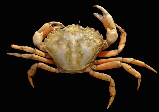
The Weldons had taken 1000 samples each with 23 attributes of wich all but the one attribute describing forehead to body length ratio seemed to follow a single normal distribution. Regarding this peculiar deviation from normal, Pearson notes:

In the case of certain biological, sociological, and economic measurements there is, however, a well-marked deviation from this normal shape, and it becomes important to determine the direction and amount of such deviation. The asymmetry may arise from the fact that the units grouped together in the measured material are not really homogeneous. It may happen that we have a mixture of \(2, 3,\dots, n\) homogeneous groups, each of which deviates about its own mean symmetrically and in a manner represented with sufficient accuracy by the normal curve.

What the paragraph describes is the problem of learning a mixture of gaussians: Each sample is drawn from one of several unknown gaussian distributions. Each distribution is selected with an unknown mixture probability. The goal is to find the parameters of each gaussian distribution as well as the mixing probabilities. Pearson focuses on the case of two gaussians which he believes is of special importance in the context of evolutionary biology:

A family probably breaks up first into two species, rather than three or more, owing to the pressure at a given time of some particular form of natural selection.

With this reasoning he stipulates that the crab measurements are drawn from a mixture of two gaussians and aims to recover the parameters of this mixture. Learning a mixture of two gaussians at the time was a formidable task that lead Pearson to come up with a powerful approach. His approach is based on the method of moments which uses the empirical moments of a distribution to distinguish between competing models. Given \(n\) samples \(x_1,...,x_n\) the \(k\)-th empirical moment is defined as \(\frac1n\sum_ix_i^k\), which for sufficiently large \({n}\) will approximate the true moment \({\mathbb{E}\,x_i^k}\). A mixture of two one-dimensional gaussians has \({5}\) parameters so one might hope that \({5}\) moments are sufficient to identify the parameters.

Pearson derived a ninth degree polynomial \({p_5}\) in the first \({5}\) moments and located the real roots of this polynomial over a carefully chosen interval. Each root gives a candidate mixture that matches the first \({5}\) moments; there were two valid solutions, among which Pearson selected the one whose \({6}\)-th moment was closest to the observed empirical \({6}\)-th moment.

Pearson goes on to evaluate this method numerically on the crab samples---by hand. In doing so he touches on a number of issues such as numerical stability and number of floating point operations that seem to me as being well ahead of their time. Pearson was clearly aware of computational constraints and optimized his algorithm to be computationally tractable.

Learning mixtures of gaussians

Pearson's seminal paper proposes a problem and a method, but it doesn't give an analysis of the method. Does the method really work on all instances or did he get lucky on the crab population? Is there any efficient method that works on all instances? The sort of theorem we would like to have is: Given \({n}\) samples from a mixture of two gaussians, we can estimate each parameter up to small additive distance in polynomial time.

Eric Price and I have a recent result that resolves this problem by giving a computationally efficient estimator that achieves an optimal bound on the number of samples:

Theorem. Denoting by \({\sigma^2}\) the overall variance of the mixture, \({\Theta(\sigma^{12})}\) samples are necessary and sufficient to estimate each parameter to constant additive distance. The estimator is computationally efficient and extends to the \({d}\)-dimensional mixture problem up to a necessary factor of \({O(\log d)}\) in the sample requirement.

Strikingly, our one-dimensional estimator turns out to be very closely related to Pearson's approach. Some extensions are needed, but I'm inclined to say that our result can be interpreted as showing that Pearson's original estimator is in fact an optimal solution to the problem he proposed.

Until a recent breakthrough result by Kalai, Moitra and Valiant (2010), no polynomial bounds for the problem were known except under stronger assumptions on the gaussian components.<

 A word about definitions

Of course, we need to be a bit more careful with the above statements. Clearly we can only hope to recover the parameters up to permutation of the two gaussian components as any permutation gives an identical mixture. Second, we cannot hope to learn the mixture probabilities in general up to small error. If, for example, the two gaussian components are indistinguishable, there is no way of learning the mixture probabilities---even though we can estimate means and variances easily by treating the distribution as one gaussian. On the other hand, if the gaussian components are distinguishable then it is not hard to estimate the mixture probabilities from the other parameters and the overall mean and variance of the mixture. For this reason it makes some sense to treat the mixture probabilities separately and focus on learning means and variances of the mixture.

Another point to keep in mind is that our notion of parameter distance should be scale-free. A reasonable goal is therefore to learn parameters \({\hat \mu_1,\hat \mu_2,\hat\sigma_1,\hat\sigma_2}\) such that if \({\mu_1,\mu_2,\sigma_1,\sigma_2}\) are the unknown parameters, there is a permutation \({\pi\colon\{1,2\}\rightarrow\{1,2\}}\) such that for all \({i\in\{1,2\},}\)

\(\displaystyle \max\left( \big|\hat\mu_i-\mu_{\pi(i)}\big|^2, \big|\hat\sigma_i^2-\sigma_{\pi(i)}^2\big|\right)\le\epsilon \cdot \sigma^2. \)

Here, \({\sigma^2}\) is the overall variance of the mixture. The definition extends to the \({d}\)-dimensional problem for suitable notion of variance (essentially the maximum variance in each coordinate) and by replacing absolute values with \({\ell_\infty}\)-norms.

Some intuition for the proof

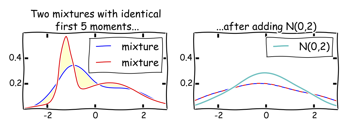
While the main difficulty in the proof is the upper bound, let's start with some intuition for why we can't hope to do better than \({\sigma^{12}}\). Just like Pearson's estimator and that of Kalai, Moitra and Valiant, our estimator is based on the first six moments of the distribution. It is not hard to show that estimating the \({k}\)-th moment up to error \({\epsilon\sigma^k}\) requires \({\Omega(1/\epsilon^2)}\) samples. Hence, learning each of the first six moments to constant error needs \({\Omega(\sigma^{12})}\) samples. This doesn't directly imply a lower bound for the mixture problem. After all, learning mixtures could be strictly easier than estimating the first six moments. Nevertheless, we know from Pearson that there are two mixtures that have matching first \({5}\) moments. This turns out to give you a huge hint as to how to prove a lower bound for the mixture problem. The key observation is that two mixtures that have matching first \({5}\) moments and constant parameters are extremely close to each other after adding a gaussian variable \({N(0,\sigma^2)}\) to both mixtures for large enought \({\sigma^2}\). Note that we still have two mixtures of gaussians after this operation and the total variance is \({O(\sigma^2).}\)

Making this statement formal requires choosing the right probability metric. In our case this turns out to be the squared Hellinger distance. Sloppily identifying distributions with density functions like only a true computer scientist would do, the squared Hellinger distance is defined as

\[\mathrm{H}^2(f,g) = \frac12\int_{-\infty}^{\infty} \Big(\sqrt{f(x)}-\sqrt{g(x)}\Big)^2 \mathrm{d}x\,. \]

Lemma. Let \({f,g}\) be mixtures with matching first \({k}\) moments and constant parameters. Let \({p,q}\) be the distributions obtained by adding \({N(0,\sigma^2)}\) to each distribution. Then, \({\mathrm{H}^2(p,q)\le O(1/\sigma^{2k+2})}\).

The lemma immediately gives the lower bound we need. Indeed, the squared Hellinger distance is sub-additive on product distributions. So, it's easy to see what happens for \({n}\) independent samples from each distribution. This can increase the squared Hellinger distance by at most a factor \({n}\). In particular, for any \({n=o(\sigma^{2k+2})}\) the squared Hellinger distance between \({n}\) samples from each distribution is at most \({o(1)}\). Owing to a useful relation between the Hellinger distance and total variation, this implies that also the total variation distance is at most \({o(1)}\). Using the definition of total variation distance, this means no estimator (efficient or not) can tell apart the two distributions from \({n=o(\sigma^{2k+2})}\) samples with constant success probability. In particular, parameter estimation is impossible.

This lemma is an example of a broader phenomenon: Matching moments plus "noise" implies tiny Hellinger distance. A great reference is Pollard's book and lecture notes. By the way, Pollard's expository writing is generally wonderful. For instance, check out his (unrelated) paper on guilt-free manipulation of conditional densities if you ever wondered about how to condition on a measure zero event without regret. Not that computer scientists are generally concerned about it.

Matching upper bound

The matching upper bound is a bit trickier. The proof uses a convenient notion of excess moments that was introduced by Pearson. You might have heard of excess kurtosis (the fourth excess moment) as it appears in the info box on every Wikipedia article about distributions. Excess moments have the appealing property that they are invariant under adding and subtracting a common term from the variance of each component.

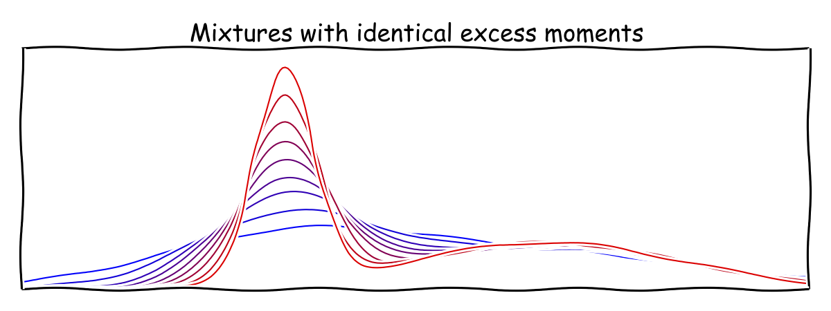
The second excess moment is always \({0.}\) As the picture suggests, we can make one component increasingly spiky and think of it as a distribution that places all its weight on a single point. In accordance with this notion of excess moments it makes sense to reparametrize the mixture in such a way that the parameters are also independent of adding and subtracting a common variance term. Assuming the overall mean of the mixture is \({0,}\) this leaves us with three free parameters \({\alpha,\beta,\gamma.}\) The third through sixth excess moment give us four equations in these three parameters.

Expressing the excess moments in terms of our new parameters \({\alpha,\beta,\gamma,}\) we can derive in a fairly natural manner a ninth degree polynomial \({p_5(y)}\) whose coefficients depend on the first \({5}\) excess moments so that \({\alpha}\) has to satisfy \({p_5(\alpha)=0.}\) The polynomial \({p_5}\) was already used by Pearson. Unfortunately, \({p_5}\) can have multiple roots and this is to be expected since \({5}\) moments are not sufficient to identify a mixture of two gaussians. Pearson computed the mixtures associated with each of the roots and threw out the invalid solutions (e.g. the ones that give imaginary variances), getting two valid mixtures that matched on the first five moments. He then chose the one whose sixth moment was closest to the observed sixth moment.

We proceed somewhat differently from Pearson after computing \({p_5}\). We derive another polynomial \({p_6}\) (depending on all six moments) and a bound \({B}\) such that \({\alpha}\) is the only solution to the system of equations

\[ \big\{p_5(y)=0,\quad p_6(y)=0,\quad 0< y\leq B\big\}. \]

This approach isn't yet robust to small perturbations in the moments; for example, if \({p_5}\) has a double root at \({\alpha}\), it may have no nearby root after perturbation. We therefore consider the polynomial \({r(y) = p_5^2(y)+p_6^2(y)}\) which we know is zero at \({\alpha.}\) We argue that \({r(y)}\) is significantly nonzero for any \({y}\) significantly far from \({\alpha}\). This is the main difficulty in the proof, but if you really read this far, it's perhaps not a bad point to switch to reading our paper.

Conclusions

I sure drooled enough over how much I like Pearson's paper. Let me conclude with a different practical thought. There were a bunch of tools (as in actual computer programs---gasp!) that made the work a lot easier. Before we proved the lower bound we had verified it using arbitrary floating point precision numerical integration to accuracy \({10^{-300}}\) for \({\sigma^2=10,100,1000,\dots}\) and the decrease in Hellinger distance was exactly what it should be. We used a Python package called mpmath for that.

Similarly, for the upper bound we used a symbolic computation package in Python called SymPy to factor various polynomials, perform substitutions and multiplications. It would've been tedious, time-consuming and error prone to do everything by hand (even if the final result is not too hard to check by hand).

To stay on top of future posts, subscribe to the RSS feed or follow me on Twitter.