Power method still powerful
The Power Method is the oldest practical method for finding the eigenvector of a matrix corresponding to the eigenvalue of largest modulus. Most of us will live to celebrate the Power Method's 100th birthday around 2029. I plan to throw a party. What's surprising is that the Power Method continues to be highly relevant in a number of recent applications in algorithms and machine learning. I see primarily two reasons for this. One is computational efficiency. The Power Method happens to be highly efficient both in terms of memory footprint and running time. A few iterations often suffice to find a good approximate solution. The second less appreciated but no less important aspect is robustness. The Power Method is quite well-behaved in the presence of noise making it an ideal candidate for a number of applications. It's also easy to modify and to extend it without breaking it. Robust algorithms live longer. The Power Method is a great example. We saw another good one before. (Hint: Gradient Descent) In this post I'll describe a very useful robust analysis of the Power Method that is not as widely known as it sould be. It characterizes the convergence behavior of the algorithm in a strong noise model and comes with a neat geometric intuition.
Power Method: Basics
Let's start from scratch. The problem that the power method solves is this:
Given \({A,}\) find the rank \({1}\) matrix \({B}\) that minimizes \({\|A-B\|_F^2.}\)
Here, \({\|A-B\|_F^2}\) is the squared Frobenius norm of the difference between \({A}\) and \({B.}\) (Recall that this is the sum of squared entries of \(A-B\)). Any rank \({1}\) matrix can of course be written as \({xy^T}\) (allowing for rectangular \({A}\)). On the face of it, this is a non-convex optimization problem and there is no a priori reason that it should be easy! Still, if we think of \({f(x,y) = \|A-xy^T\|_F^2}\) as our objective function, we can check that setting the gradient of \({f}\) with respect to \({x}\) to zero gives us the equation by \({x=Ay}\) provided that we normalized \({y}\) to be a unit vector. Likewise taking the gradient of \({f}\) with respect to \({y}\) after normalizing \({x}\) to have unit norm leads to the equation \(y={A^T x.}\) The Power Method is the simple algorithm which repeatedly performs these update steps. As an aside, this idea of solving a non-convex low-rank optimization problem via alternating minimization steps is a powerful heuristic for a number of related problems.
For simplicity from here on we'll assume that \({A}\) is symmetric. In this case there is only one update rule: \({x_{t+1} = Ax_{t}.}\) It is also prudent to normalize \({x_t}\) after each step by dividing the vector by its norm.
The same derivation of the Power Method applies to the more general problem: Given a symmetric \({n\times n}\) matrix \({A,}\) find the rank \({k}\) matrix \({B}\) that minimizes \({\|A-B\|_F^2}\). Note that the optimal rank \({k}\) matrix is also given by the a truncated singular value decomposition of \({A.}\) Hence, the problem is equivalent to finding the first \({k}\) singular vectors of \({A.}\)
A symmetric rank \({k}\) matrix can be written as \({B= XX^T}\) where \({X}\) is an \({n\times k}\) matrix. The update rule is therefore \({X_{t+1} = AX_{t}}\). There are multiple ways to normalize \({X_t}\). The one we choose here is to ensure that \({X_t}\) has orthonormal columns. That is each column has unit norm and is orthogonal to the other columns. This is can be done using good ol' boys Gram-Schmidt (though in practice people prefer the Householder method).
The resulting algorithm is often called Subspace Iteration. I like this name. It stresses the point that the only thing that will matter to us is the subspace spanned by the columns of \({X_t}\) and not the particular basis that the algorithm happens to produce. This viewpoint is important in the analysis of the algorithm that we'll see next.
A Robust Geometric Analysis of Subspace Iteration
Most of us know one analysis of the power method. You write your vector \({x_t}\) in the eigenbasis of \({A}\) and keep track of how matrix vector multiplication manipulates the coefficients of the vector in this basis. It works and it's simple, but it has a couple of issues. First, it doesn't generalize easily to the case of Subspace Iteration. Second, it becomes messy in the presence of errors. So what is a better way? What I'm going to describe was possibly done by numerical analysts in the sixties before the community moved on to analyze more modern eigenvalue methods.
Principal Angles
To understand what happens in Subspace Iteration at each step, it'll be helpful to have a potential function and to understand under which circumstances it decreases. As argued before the potential function should be basis free to avoid syntactic arguments. The tool we're going to use is the principal angle between subspaces. Before we see a formal definition, it turns out that much of what's true for the angle between two vectors can be lifted to the case of subspaces of equal dimension. In fact, much of what's true for the angle between spaces of equal dimension generalizes to unequal dimensions with some extra care.
The two subspaces we want to compare are the space spanned by the \({k}\) columns of \({X_t}\) and the space \({U}\) spanned by the \({r}\) dominant singular vectors of \({A.}\) For now, we'll discuss the case where \({r=k.}\) I'll be a bit sloppy in my notation and use the letters \({U,X_t}\) for these subspaces.
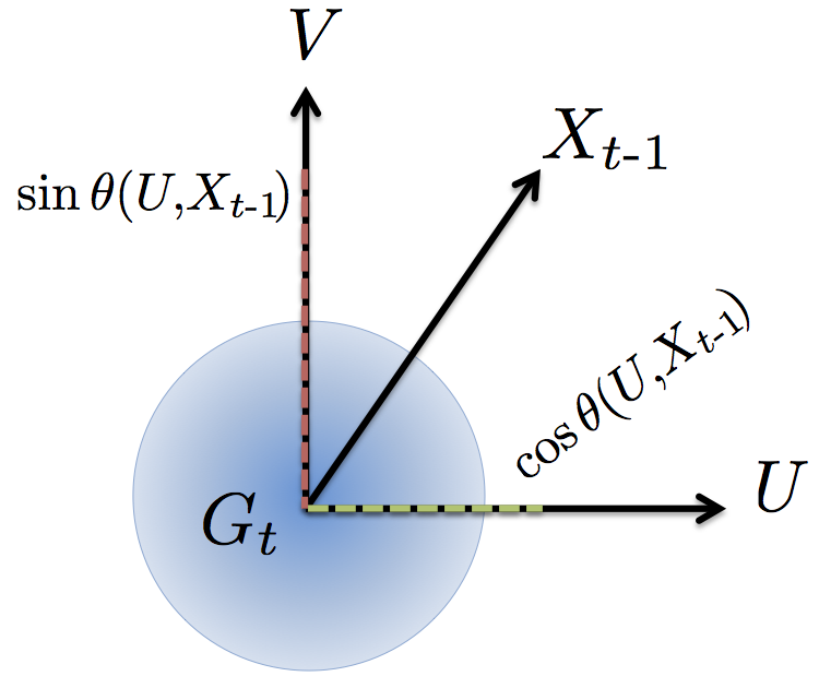
Let's start with \({k=1}\). Here the cosine of the angle \({\theta}\) between the two unit vectors \({X_t}\) and \({U}\) is of course defined as \({\cos\theta(U,X_t)= |U^T X_t|.}\) It turns out that the natural generalization for \({k>1}\) is to define
\(\displaystyle \cos\theta(U,X_t)=\sigma_{\mathrm{min}}(U^T X_t). \)
In words, the cosine of the angle between \({U}\) and \({X_t}\) is the smallest singular value of the \({k\times k}\) matrix \({U^T X_t}\). Here's a sanity check on our definition. If the smallest singular value is \({0}\) then there is a nonzero vector in the range of the matrix \({X_t}\) that is orthogonal to the range of \({U}\). In an intuitive sense this shows that the subspaces are quite dissimilar. To get some more intuition, consider a basis \({V}\) for the orthogonal complement of \({U.}\) It makes sense to define \({\sin\theta(U,X_t)= \sigma_{\mathrm{max}}(V^T X_t)}\). Indeed, we can convince ourselves that this satisfies the familiar rule \({1= \sin^2\theta + \cos^2\theta}\). Finally, we define \({\tan\theta}\) as the ratio of sine to cosine.
A strong noise model
Let's be ambitious and analyze Subspace Iteration in a strong noise model. It turns out that this will not actually make the analysis a lot harder, but a lot more general. The noise model I like is one in which each matrix-vector product is followed by the addition of a possibly adversarial noise term. Specifically, the only way we can access the matrix \(A\) is through an operation of the form
\(\displaystyle Y = AX + G. \)
Here, \({X}\) is what we get to choose and \({G}\) is the noise matrix we may not get to choose. We assume that \(G$ is the only source of error and that arithmetic is exact. In this model our algorithm proceeds as follows:
- \({Y_t = AX_{t-1} + G_t}\)
- \({X_t = \text{Orthonormalize}(Y_t)}\)
The main geometric lemma
To analyze the above algorithm, we will consider the potential function \({\tan\theta(U,X_t).}\) If we pick \({X_0}\) randomly it's not so hard to show that it starts out being something like \({O(\sqrt{kn})}\) with high probability. We'll argue that \({\tan\theta(U,X_t)}\) decreases geometrically at the rate of \({\sigma_{k+1}/\sigma_{k}}\) under some assumptions on \({G_t}\). Here, \({\sigma_k}\) is the \({k}\)-th largest singular value. The analysis therefore requires a separation between \({\sigma_k}\) and \({\sigma_{k+1}}\). (NB: We can get around that by taking the dimension \({r}\) of \({U}\) to be larger than \({k.}\) In that case we'd get a convergence rate of the form \({\sigma_{r+1}/\sigma_k.}\) The argument is a bit more complicated, but can be found here.)
Now the lemma we'll prove is this:
Lemma. For every \({t\ge 1,}\)
\(\displaystyle \tan\theta(U,X_t) \le \frac{\sigma_{k+1}\sin\theta(U,X_{t-1})+\|V^T G_t\|} {\sigma_k\cos\theta(U,X_{t-1})-\|U^T G_t\|}. \)
This lemma is quite neat. First of all if \({G_t=0,}\) then we recover the noise-free convergence rate of Subspace Iteration that I claimed above. Second what this lemma tells us is that the sine of the angle between \({U}\) and \({X_{t-1}}\) gets perturbed by the norm of the projection of \({G_t}\) onto \({V}\), the orthogonal complement of \({U.}\) This should not surprise us, since \({\sin\theta(U,X_{t-1})=\|V^T X_{t-1}\|.}\) Similarly, the cosine of the angle is only perturbed by the projection of \({G_t}\) onto \({U.}\) This again seems intuitive given the definition of the cosine. An important consequence is this. Initially, the cosine between \({U}\) and \({X_0}\) might be very small, e.g. \({\Omega(\sqrt{k/n})}\) if we pick \({X_0}\) randomly. Fortunately, the cosine is only affected by a \({k}\)-dimensional projection of \({G_t}\) which we expect to be much smaller than the total norm of \({G_t.}\)
The lemma has an intuitive geometric interpretation expressed in the following picture:
It's straightforward to prove the lemma when \({k=1}\). We simply write out the definition on the left hand side, plug in the update rule that generated \({X_t}\) and observe that the normalization terms in the numerator and denominator cancel. This leaves us with the stated expression after some simple manipulations. For larger dimension we might be troubled by the fact that we applied the Gram-Schmidt algorithm. Why would that cancel out? Interestingly it does. Here's why. The tangent satisfies the identity:
\(\displaystyle \tan\theta(U,X_t) = \|(V^T X_t)(U^TX_t)^{-1}\|. \)
It's perhaps not obvious, but not more than an exercise to check this. On the other hand, \({X_t = Y_t R}\) for some invertible linear transformation \({R.}\) This is a property of orthonormalization. Namely, \({X_t}\) and \({Y_t}\) must have the same range. But \({(U^TY_tR)^{-1}=R^{-1}(U^T Y_t)^{-1}}\). Hence
\(\displaystyle \|(V^T X_t)(U^TX_t)^{-1}\| = \|(V^T Y_t)(U^TY_t)^{-1}\|. \)
It's now easy to proceed. First, by the submultiplicativity of the spectral norm,
\(\displaystyle \|(V^T Y_t)(U^TY_t)^{-1}\| \le \|(V^T Y_t)\|\cdot\|(U^TY_t)^{-1}\|. \)
Consider the first term on the right hand side. We can bound it as follows:
\(\displaystyle \|(V^T Y_t)\|\!\le\!\|V^TAX_{t-1}\| + \|V^T G_t\|\!\le\! \sigma_{k+1}\sin\theta(U,X_{t-1}) + \|V^T G_t\|. \)
Here we used that the operation \({V^T A}\) eliminates the first \({k}\) singular vectors of \({A.}\) The resulting matrix has spectral norm at most \({\sigma_{k+1}}\).
The second term follows similarly. We have \({\|(U^T Y_t)^{-1}\| = 1/\sigma_{\mathrm{min}}(U^TY_t)}\) and
\(\displaystyle\!\!\!\sigma_{\mathrm{min}}(U^TY_{t})\!\ge\!\sigma_{\mathrm{min}}(U^TAX_{t-1})\!-\!\|U^T G_t\|\!\ge\! \sigma_k\cos\theta(U,X_{t-1})\!-\!\|U^T G_t\|\!\!\!\)
This concludes the proof of the lemma.
Applications and Pointers
It's been a long post, but it'd be a shame not to mention some applications. There are primarily three applications that sparked my interest in the robustness of the Power Method.
The first application is in privacy-preserving singular vector computation. Here the goal is to compute the dominant singular vectors of a matrix without leaking too much information about individual entries of the matrix. We can formalize this constraint using the notion of Differential Privacy. To get a differentially private version of the Power Method we must add a significant amount of Gaussian noise at each step. To get tight error bounds it's essential to distinguish between the projections of the noise term onto the space spanned by the top singular vectors and its orthogonal complement. You can see the full analysis here.
Another exciting motivation comes from the area of Matrix Completion. Here, we only see a subsample of the matrix \({A}\) and we wish to compute its dominant singular vectors from this subsample. Alternating Minimization (as briefly mentioned above) is a popular and successful heuristic in this setting, but rather difficult to analyze. Jain, Netrapalli and Sanghavi observed that it can be seen and analyzed as an instance of the noisy power method that we discussed here. The error term in this case arises because we only see a subsample of the matrix and cannot evaluate exact inner products with \({A.}\) These observations lead to rigorous convergence bounds for Alternating Minimization. I recently posted some improvements.
Surprisingly, there's a fascinating connection between the privacy setting and the matrix completion setting. In both cases the fundamental parameter that controls the error rate is the coherence of the matrix \({A}\). Arguing about the coherence of various intermediate solutions in the Power Method is a non-trivial issue that arises in both settings and is beyond the scope of this post.
Finally, there are very interesting tensor generalizations of the Power Method and robustness continues to be a key concern. See, for example, here and here. These tensor methods have a number of applications in algorithms and machine learning that are becoming increasingly relevant. While there has been some progress, I think it is fair to say that much remains to be understood in the tensor case. I may decide to work on this once my fear of tensor notation recedes to bearable levels.