The geometric view on sparse recovery
Sparsity is of fundamental importance in much of signal processing, optimization, computer science and statistics. It was also a major theme in both workshops so far in the Simons Big Data program. The second workshop on succinct representations ended a few weeks ago. Those still barely conscious after a week of technical talks were rewarded by this sunset over Berkeley. (Technically, you still would have had to climb up to the top of Centennial Dr somehow.)
Sparsity is a solution concept and not just a technical term. Sparse solutions to an optimization problem are often more well-behaved as they explain a phenomenon with fewer parameters. In high-dimensional settings where there are more variables than constraints, enforcing sparsity makes sense of problems that would otherwise be underdetermined.
There's been so much work on sparsity it seems hard to find a place to start. Fortunately, there's a simple and elegant---yet powerful---geometric approach underlying many results in sparse recovery that I'll focus on here.
The Basic Picture
Perhaps the simplest example is solving an underdetermined system of linear equations \({Ax=b.}\) Assume \({A}\) is an \({m\times n}\) matrix and \({b=Ax_0}\) for some \({k}\)-sparse vector \({x_0}\) (i.e., \({x_0}\) has at most \({k}\) nonzero entries). We can hope to recover \({x_0}\) provided that \({A}\) has more than \({k}\) linearly independent rows. How do we do this efficiently? The problem of solving \({Ax=b}\) s.t. \({x}\) is \({k}\)-sparse is NP-hard. We will instead consider the problem
\(\displaystyle \min f(x)\quad\mathrm{s.t.}\,\, Ax=b \)
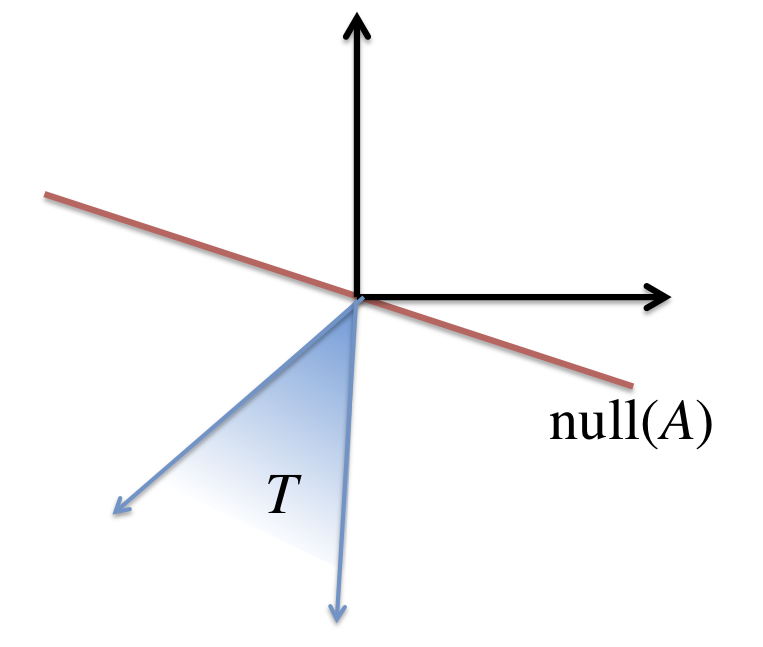
for some convex function \({f\colon\mathbb{R}^n\rightarrow\mathbb{R}.}\) The function \({f}\) has no easy job. It needs to favor sparse solutions and yet be convex! Why should such a creature exist? Let's think about what we're asking for formally. We know that all the solutions to \({Ax=b}\) can be written as \({x_0+h}\) where \({h}\) is in the null space of \({A}\). Hence, \({x_0}\) is the solution to our problem if for all \({h}\) in the null space of \({A,}\) we have \({f(x_0+h) > f(x_0).}\) Consider therefore the set of all directions that would actually decrease the function value. These directions form a cone, called tangent cone, formally defined as:
\(\displaystyle T(x_0) = \{ d \colon \exists \alpha>0\quad f(x_0 + \alpha d) \le f(x_0) \}. \)
The Restricted Nullspace Property
The central geometric question can then be phrased as: When is it the case that the tangent cone intersects the nullspace only at the origin? Formally, we're asking:
\(T(x_0)\cap \mathrm{null}(A)=\{ 0 \}\quad \)?
Restricted Nullspace Property is actually the name of a closely related property. Nevertheless I decided to run with this name for the purpose of this blog post.
It is helpful to think of \({\mathrm{null}(A)}\) as a random subspace. This happens, for example, when \({A}\) is a random Gaussian matrix. On intuitive grounds, we should aim to make \({T(x_0)}\) as "small" as possible to avoid any non-trivial intersection with the random nullspace while maintaining convexity. A natural choice is to let \({f}\) be the familiar \({\ell_1}\)-norm \({f(x)=\|x\|_1.}\) Even with these two choices though it's not obvious how to analyze the intersection of tangent cone and nullspace. We'd have to argue about all points in the tangent cone. You can probably guess what's next. Instead of proving the condition directly, we'll exhibit a "dual certificate". Duality is really easy here. The negative of the dual cone of \({T(x_0)}\) is the set
\(\displaystyle G = \{ g \colon f(y) \ge f(x_0) + \langle g,y-x\rangle \}. \)
If \({f}\) were differentiable at \({x_0,}\) then \({G}\) would be the singleton set containing the gradient of \({f}\) at \({x_0.}\) Since this is not the case for the \({\ell_1}\)-norm, there is an entire cone of vectors satisfying the relation. This cone is often called the subdifferential of the \({\ell_1}\)-norm at \({x_0.}\) Its members are called subgradients.
Now, suppose we had a vector \({g\in G}\) such that \({g}\) was a linear combination of the rows of \({A,}\) i.e., \({g = A^t \lambda}\) for some vector \({\lambda.}\) In this case, for all \({y=x_0+h}\) with \({h}\) in the null space of \({A,}\) it must be the case that
\(\displaystyle f(y) \ge f(x_0) + (A^t\lambda)^t (y-x_0) = f(x_0) + \lambda^t(Ah) = f(x_0). \)
In other words, such a vector \({g}\) would certify the optimality of \({x_0.}\)
What we've done so far has just been basic convex analysis and holds in great generality. Nevertheless, it makes sense to internalize this Ansatz as it is the starting point of many results in the area. (Note also my flawless command of the German language. Only Eric Price argues that I misuse the term.)
Construction of the Dual Certificate
Let's see why this approach is powerful. First, the subdifferential of the \({\ell_1}\)-norm is easy to characterize. Using some basic rules it turns out that \({G}\) contains all the vectors \({g}\) such that:
1. \({g_i}\) equals the sign of \({(x_0)_i}\) for all \({i}\) in the support of \({x_0}\) which we'll denote by \({S,}\) and
2. \({g_i\in[-1,1]}\) for all \({i\in S^c.}\)
So, the first condition is a set of \({|S|}\) linear equations on \({A^t\lambda.}\) Since \({A}\) has more than \({|S|}\) rows and a random Gaussian matrix is in general position, this set of equations has a solution! The second constraint bounds the \({\ell_\infty}\)-norm of \({A^t\lambda}\) outside the support of \({x_0.}\)
Remarkably, the way people find a suitable \({\lambda}\) is by solving, again, a convex optimization problem! In this case, we're going to find the least squares solution to (1) and hope that magically it will satisfy (2). Actually, there isn't too much magic. A reason for this choice is this. Suppose we partition the columns of \({A}\) as \({A = [ A_1 | A_2 ]}\) according to the support of \({x_0.}\) For simplicity we assume that the support is on the first \({|S|}\) columns of \({A.}\) The least squares solution has the following appealing property. Of course, it satisfies the linear equations on \({A_1}\). Moreover, the \({\ell_\infty}\)-norm of \({A_2^t \lambda}\) is dictated by the \({\ell_2}\)-norm of \({\lambda}\). This is because \({A_1}\) and \({A_2}\) are statistically independent and \({A_2}\) is distributed as a random Gaussian matrix. This interpretation of why least squares is conceptually the right thing to look at in the Gaussian case was pointed out to me by Sushant Sachdeva.
What's left is to use some probability theory to work out the parameters that we get. For those details check out Ben Recht's talk here.
The Issue of Noise
Alas, the picture isn't quite as simple as suggested so far. In almost any realistic setting we'd like sparse recovery to be robust to noisy observations. This leads to several problems that are beyond the scope of this blog post. In the case of linear equations this leads to the theory of the \({\ell_1}\)-regularized least squares, usually called LASSO. Here the goal is to minimize a least squares error, while controlling the \({\ell_1}\)-norm of the solution. Martin Wainwright's first talk at the Big Data Boot Camp dealt with the theory of LASSO in detail.
From Vectors to Matrices: Matrix Sensing and Completion
Much of what we discussed is still true when we go from vectors to matrices. All concepts generalize by looking at the spectrum of the matrix. Sparsity in the spectrum means low rank. The \({\ell_1}\)-norm applied to the spectrum of the matrix is called nuclear norm and plays a crucial role in the matrix world. The generalization of the above proof is most direct in the case of Matrix Sensing. Here we are given linear measurements on a matrix \({ {\cal A}(X) = B}\) where \({B={\cal A}(X_0)}\) and \({X_0}\) is a low-rank matrix. Just to be clear, \({ {\cal A}}\) is now a linear operator on matrices. One could define a random Gaussian operator by taking inner products between random Gaussian matrices and the matrix \({X.}\)
A particularly well-studied linear operator is the subsampling operator. It takes \({X}\) and projects its entries to some subset \({\Omega.}\) Recovering \({X_0}\) in this case is known as Matrix Completion. It's a noticeably more difficult problem. Even if \({\Omega}\) is nice, say, uniformly random of some density, the approach can't work if \({X_0}\) hides its support in a tiny subset of the matrix. That's why we need additional assumptions. The prevailing assumption is known as incoherence. It states that the singular vectors of \({X_0}\) should be de-localized in the sense of having small inner product with the standard basis. This rules out the pathological example I just mentioned.
Incoherence is often justified by saying that otherwise unique recovery were simply not possible. Why should we insist on uniquely recovering a solution? In many cases it might be interesting to find any low-rank matrix consistent with the observations. Much less is known about matrix completion without an incoherence assumption in the regime where unique recovery is not possible. As far as I know, there are neither convincing hardness results (apart from NP-hardness in full generality) nor strong positive results.
Other Pointers
I've only touched on the subject lightly. There is much more to say and several talks I haven't mentioned. Here are some:
- Sometimes the \({\ell_1}\)-norm is just too simple and ignores the structure of the problem in a particular application. Francis Bach spoke about using submodular functions instead of the \({\ell_1}\)-norm. The Lovasz extension leads to a convex relaxation that makes the approach feasible.
- Sparsity also makes sense in settings where the signal has no coordinate structure. An example is Spectrum Estimation where the observations are combinations of few sinusoids. One could hack this application by some discretization, but a more elegant solution is possible. This was yet another talk by Ben Recht.
- Martin Wainwright's second talk at the Boot Camp showed a very appealing general statistical framework for reasoning about regularized convex optimization.
To follow future posts, it’s probably best to subscribe to the RSS feed or follow me on Twitter. It's some web site that theoreticians don't use.